
HOW TO CONTROL THE NORTH AREA BEAM LINESThe North Area beams H2, H4, H6, H8, P42, K12 and M2 are produced by a high-intensity primary proton beam, impinging on each of the three primary targets T2, T4 or T6. The ‘useful’ particles are picked up by the beam lines and are transported to the user areas. These beam lines are long (from about 500 to almost 1200 meters) and complex and contain a large number of elements of different natures, such as targets, magnets, collimators, dumps, absorbers, converters, detectors, vacuum pumps and access doors.
Each equipment has its own settings and readings, which depend on the required operational mode, on the beam momentum, on the wanted intensity and particle type, on the state of the access to the areas on the beam line and sometimes even on the settings in neighboring beam lines. Most of these settings can be managed by the users themselves via the ‘Cesar’ application for beam line control[1]. A very succinct description of this software is given in section 2. Detailed instructions concerning the general features of the Cesar application are available in a separate document. In the present document we rather address in a general way the most common tasks and how they are best performed.
Every beam line has been designed with specific main purposes and strong
points and therefore the detailed use of the beam lines is different for
each of them. The specificities of each beam line are normally described
in a specific User Manual for the beam line. Information can of course
also be obtained from the AB/ATB/SBA beam line expert for the beam in
question.
This document is organized in 11 sections
IntroductionBefore starting to modify settings in a beam line, it is of obvious importance to know what one wants to achieve and what equipment one needs to act on. This information is usually obtained from the information available on the SBA web pages, from the beam line experts or SPS operators or from the more experienced beam line users in your experiment. Particularly useful documents are
 Figure 1: Synoptical diagram of the North Area beam lines Your beam line is a complex system that picks up particles emerging from
the primary target and makes a selection in terms of momentum and angle.
The so-called “wobbling station”, described in section 3, ensures that
sufficient particles of the requested type and energy are sent towards
your beam line in a way consistent with the requirements of the other
beam lines derived from the same primary target. Dipole magnets, called Bends, are used to guide the particles
through the tunnels towards the relevant experimental areas and also to
introduce dispersion, necessary to achieve momentum selection. Trims
are small dipoles that have no nominal deflection angles but allow
corrections to the beam steering. Quadrupoles help to control the
beam size and dispersion along the beam line. Together with (adjustable)
slits, called Collimators, they define the acceptance of the beam
line in momentum bite and angle. The settings of these elements are
collected in so-called beam files, described in section 4. The settings
and control of magnets and collimators are described in sections 5 and
6. The amount of hadrons as well as the relative abundance of pions, kaons
and protons can be calculated with the
partprod program.
This program calculates the intensity and composition of the secondary
beam. Various absorbers, converters and secondary targets allow to
control the beam composition and intensities taking advantage of
interactions or Bremsstrahlung in their material. In that case the
energy of the beam leaving the absorber or secondary target is typically
significantly lower than the secondary beam momentum. This must be taken
correctly into account in the magnet settings and hence in the beam
files. The control of absorbers, converters and secondary targets is
described in section 7. Several types of detectors allow checks of beam intensities and the beam
spot along the beam line and consequently also to correct and optimize
the beam steering and focusing. These detector types comprise
scintillators, various types of wire chambers and filament scanners.
Cerenkov counters provide particle identification. Details of their use
are given in section 8. Dumps are essential parts of the safety system of the beam lines. In
case of access to your experimental area the beam must imperatively be
stopped by moving dumps into the beam and or switching off a number of
well-defined dipole magnets. In special cases other elements such as
primary targets are part of the safety chains, too. Your personal safety
is guaranteed by the access system, which is implemented mostly in
hardware. However, the beam line must be configured especially for
either access or beam. The software tools to achieve this are described
in section 9. The beam from the SPS is delivered in so-called super-cycles. The
super-cycle configuration changes rather frequently. The presently
active super-cycle and its properties are shown on the so-called
page-1 screens that are
available in most control rooms as well as
on the web. The super cycle contains one or more ‘flat tops’,
typically 4.8 or 9.6 seconds long, during which beam is extracted
towards the North Area targets with a time distribution as uniform as
possible, in principle without RF structure. In between flat tops the
SPS is used to inject and accelerate the beam or to provide beams to
other users (CNGS, LHC, machine studies, …). A detailed planning of
super-cycles can be found on the
SPS Coordinator’s schedule
web
pages. Many programs are synchronized with particular timing
‘events’ in the super-cycle, such as the start or end of the flat top.
Magnet currents are typically refreshed only at the start of the flat
top, whereas detector readings are typically only updated after the end
of each flat top. The page-1 screen also allows you to check easily
whether or not the SPS is providing beam. Even when there is beam
extracted from the SPS onto your primary target, it may happen that
there is no beam arriving in your experiment. Section 10 describes some
tools and techniques to find out whether there is beam or not in your
area and why. Finally we conclude in section 11, which gives some hints on what to do
if everything else fails. 2 - A short overview of the Cesar application softwareAs explained in the
Cesar
documentation, the Cesar application starts automatically on the
beam terminals in the experiment control rooms after booting. The Cesar
GUI is shown in Figure 2.  Figure 2:The Cesar application window
Settings can be verified or changed via several mechanisms:
Just below the task button bar, you find a list of ‘work spaces’,
corresponding to individual beam lines. In the user barracks, normally
only one work space is accessible. In the central control rooms, please
make sure you have selected correctly the work space tab corresponding
to your beam line. 3 - What is a wobbling station?As seen in Figure 1, two beam lines (H2 and H4) are derived
simultaneously from the T2 primary target. Similarly up to three beams
are running simultaneously via the T4 target. Each beam line has its own
requirements in terms of beam momentum, charge (positive or negative)
and intensities. On top of that, these requirements change frequently
with time. The required
flexibility is provided by the so-called ‘wobbling stations’. As an
example we show in Figure 3 the T2 wobbling station for one specific
setting, namely +150 GeV/c secondary hadrons in H2 and -150 GeV/c
hadrons in H4. In order to achieve this, two sets of dipoles just upstream of the
target, B1T and B2T, direct the beam towards the center of a third set
of dipoles B3T, located a few meters downstream of the target. The H2
and H4 beam lines start from the center of B3T at different angles. In
this particular case the protons follow the bisector between the H2 and
H4 axes. The B3T dipoles are set to sweep +150 and -150 GeV/c particles
from that bisector into the H2 and H4 beam lines, where they pass
through relatively small holes in special thick dump-collimators called
TAXes. Different momentum particles, including the primary protons
traversing the target, hit the TAX at different positions, where there
is no hole, so that they are cleanly dumped[2].
The monitors TBIU and TBID (Upstream and Downstream of the target) that
allow the steering of the protons onto the primary target are displaced
onto the calculated nominal trajectory of the primary proton beam. By changing the orientation of the proton beam or selecting particles
with non-zero production angle, a large number of requirements can be
met. An alternative option is to use a strong field in B3T to sweep away
all charged particles from the TAX holes and to send only neutral
particles through the holes. The beam lines are set to either pick up
pions of protons from Ko or Lambda decays or electrons from
conversion of photons in a lead converter located just behind the TAX.
 Figure 3: The T2 wobbling station with positive hadrons in H2 and negatives in H4 The settings of the H2 and H4 beam lines must be matched to the wobbling
station settings. Not only the beam momenta must match, but also
production angles and angular offsets (‘skew’) of the beam through the
TAX hole with respect to the nominal beam direction must be correctly
taken into account. A similar system exists for the T4 target, but in this case 3 beam lines
share the same target and the
constraints are stronger. T6 has no wobbling station, the momentum ratio between the P61 and M2
lines is fixed to exactly ‑2.0, e.g. 400 GeV/c primary beam in P61 (i.e.
P0 from T6) implies -200 GeV/c momentum in M2. The settings of the wobbling stations are agreed at the weekly schedule
meetings and are prepared by the responsible beam physicists and
executed by the SPS operation teams. 4 - Reference settings and Beam FilesThe most frequently changing settings of beam elements are magnet
currents and collimator openings. E.g. in the M2 beam line there are 67
magnet currents (11 bends, 7 trims, 36 groups of quadrupoles, 9 magnetic
collimators and 4 MIBs) and 18 collimator motor positions (for 9
collimators). The management of these settings would be virtually
impossible without using so-called ‘beam files’ containing well defined
and valid reference settings. Separate files exist for different beam
momenta and for secondary and tertiary beams. Often different files
exist for electron, hadron and muon beams. Different wobbling
configurations will often require different files for the beam lines
behind. On top of that different users have different beam zones and
different beam requirements. For all those reasons there may be many
files for a single beam line. Not all of them may work in a given
situation!
The list of available beam files can be inspected by invoking the
Beam File Browser. This can be done by either clicking on the
Browsertask button or by selecting
in the menu Files →Browse. The Files Menu also
provides options to only show files compatible with the active wobbling
settings (‘Browse beam files filtered by wobbling’) or files for your specific
experiment or zone (‘Browse by Experiment’). An example of a Beam File Browser window is
shown in Figure 4. 4.1 Producing filesFiles can be produced – painfully – by hand via the
View or Edit
commands in the
Files menu. Normally this should
be done by the expert beam physicists. For small modifications the user
can also do it. The View command allows modifying settings one by one
(select a current of collimator, select ‘Write
to File Reference’ and enter the new value). It also allows
modification of the file name. The
Edit command is more convenient when there are many changes,
but it invokes separate spreadsheet programs (Do not forget to send the
edited values to the database at the end!). In practice it is more
convenient to save the current reference settings to a beam file using
the ‘BeamRefs
→ Selected File’ button. 4.2 Loading filesA selected file can be activated by using the Load Beamfile button. You are then offered the choice to apply the settings for magnets or collimators or both. The program will then send the new reference currents and positions to the hardware and to the BeamReference for each equipment.If some settings have not been reached successfully, the user is informed of this. Please confirm ‘Yes’ that you want to continue loading the file and take corrective action (see sections 5 and 6). Please do not forget to check in detail the status of magnets and collimators after loading a file! 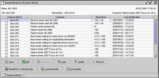 Figure 4: The Beam File Browser window
4.3 Saving new settings into a fileOnce the beam file values have been successfully loaded, the user may change individual settings (see sections 5 and 6), in which case the BeamRef settings become different from the Beam File values (indicated by ‘F’ in the corresponding status column). If the new settings are considered better than the file, the beam file may be updated via the ‘BeamRefs→ Selected File’ button.4.4 Momentum extrapolationFiles with the same characteristics but at different momentum may be
produced automatically from a selected reference file by using the
Extrapolate button. Specify the number of the new file (it
must be new, the program does not allow to overwrite an existing file!),
the new secondary beam momentum. Special algorithms exist for
high-energy electron files (above ~100 to 150 GeV/c) where the energy
loss of electrons due to synchrotron radiation must be taken into
account: choose the appropriate option, e.g.
Hadron => Electron. A special situation occurs for tertiary beams, where the upstream part
of the beam has a well-defined beam momentum and the part downstream of
an intermediate target has a lower momentum. In that case you must
indicate at which element the momentum change occurs (ask the beam line
expert) and what the tertiary beam momentum shall be. 4.5 Beam File managementSpecial buttons have been provided to Delete or
Copy files. You may also select two or more files and Compare them. 5 - Beam steering, focusing and control of magnetsBeam steering and focusing of a beam line are controlled by different kinds of magnets:
5.1 Status and setting of magnetsThe status of the magnets is obtained via the
Status
→ Magnets
menu or via the
Magnet Status
task button. The status of individual magnets can be obtained by
double clicking on the name(s) of the magnet(s) in the physicist tree.
The status panel shows the current reading and the current BeamRef
setting for each magnet. If the run button at the bottom is activated,
these readings are refreshed at every start of flat top, either for the
selected (highlighted) magnets in the panel or for all of them. Also
indicated are the maximum allowed current, some special information and
comments, including error condition reports. The error reports are
shortcuts and rather cryptical for the non-initiated; a more verbose
display is obtained with the ‘Display
Faults’ option. 5.2 Correcting problems with magnets and rectifiersThe rectifier (power supply) status is a more expert oriented
application than the magnet status. It has no link to beam file
references, but allows more actions than the magnet status. It can be
invoked from the magnet status or from the ‘Rectifier
Status’ task button or from
the menu via
Status
→ Rectifier Status. Buttons
allow to
Reset a rectifier (clear
faults), switch it on or off, to put it in standby mode or simply to set
a current. In general it is recommended
not to switch rectifiers
OFF,
but put them in
STANDBY mode, except if the
rectifier will be stopped for very long periods (e.g. many days).
Sometimes, if a rectifier does
not start, it may unblock the situation if you try the opposite polarity
first and then switch to the correct polarity once the rectifier works
again. It is not possible to start a rectifier as long as the faults have not
been reset. If you do not succeed to reset the faults or if nothing else
helps: please call the SPS operator. There is also an option to switch a rectifier from
PULSED to
DC mode or vice versa. In pulsed
mode the rectifier only powers the magnet during the flat top. At very
low currents this may lead to instabilities. On the other hand at high
currents the DC mode may lead to overheating of the magnets. In general
it is not recommended to change this setting without consulting the
operators or your beam line expert (i.e. only if you know what you are
doing). 5.3 Degaussing of magnetsThe degauss program can be useful in case it is very important to guarantee absolute precision in the absolute momentum scale. This is e.g. the case for linearity studies of calorimeters. This program cycles through a number of current settings for all or a number of selected power supplies. The inconvenience is that it is a somewhat lengthy process and the risk of equipment failure is not negligible in case you degauss many magnets at the time. It is invoked by a right-hand button mouse click on the magnet(s) selected in the Magnet Status. A contextual menu appears in which you can select the Degauss option. Two strategies are proposed:
5.4 Other useful commandsIn the contextual menu you will also find two other useful options:
6 - Beam intensity, momentum spread and control of collimatorsCollimators are adjustable slits, that define the acceptance of the beam line in angle and/or momentum, depending on their location in terms of beam line optics.In the North Area optics drawings, red curves indicate the trajectory of a particle produced at an angle with respect to the nominal beam optics. This is also called the sine-like wave or R12, resp R34 term. When that line crosses the axis, the beam has a so-called focus in that point. Normally the beam momentum and momentum bite are defined by a collimator located in a ‘dispersive focus’, i.e. a focus where the dispersion (the blue dotted line in the optics drawing) is large. Such a collimator is called a momentum slit. The beam flux is normally nicely proportional with the opening of a momentum slit, but the momentum spread as well. Acceptance collimators are located in a place where the sine-like wave is large. It defines the angular range that can be accepted by the beam line. The beam flux increases with acceptance angle, but in a non-linear way. In many cases the optics is arranged such that there is a non-dispersive focus at your experiment. If that is the case, the beam spot is to first order independent of the openings of acceptance and momentum slits. However, the beam divergence does increase with larger openings. In case the beam is parallel or if there is strong dispersion at your experiment, the beam spot will rapidly increase with larger collimator openings. 6.1 Collimator controlCollimator gaps can be observed or changed with the Collimator Status
application, that can be invoked using the
Collimator Status task button
or via the Status → Collimator
menu. The collimator has two jaws, which both must have a
position between the min and max positions indicated in the status
panel. Jaw 2 must be at a more positive position than Jaw 1 and the
minimum opening is about 1 mm. Normally a collimator is considered wide
open with an aperture of ±40 mm (or more), beyond which other apertures
usually take over. There are some exceptions, notably collimator 5 in
the M2 beam which can be opened to ±100 mm. Collimators can act in the
horizontal or vertical plane; this is indicated in the status panel. 6.2 Loading of collimator settingsIt is of course also possible to go back to the collimator settings from the original beam file by loading the beam files (via the File Browser application) for the collimators only.7 - The type of particles in your beam line: absorbers, converters, etceteraThe type of particles in your beam line depends on many parameters and on specific properties of your beam line. Nevertheless there are some general features.First one should distinguish between various basic operational modes:
7.1 Secondary beam modeSecondary beams are normally mixed beams, i.e. a mixture of different hadron species plus some amount of electrons (or positrons). In most beam lines an ‘absorber’ can be moved onto the beam to remove an electron component. This absorber is located somewhere half along the beam line in a focus in both planes. This absorber is almost (but not quite) transparent to hadrons, but most of the electrons loose a substantial fraction of their energy in it due to Bremsstrahlung. Those degraded electrons will not be transported by the second part of the beam line and are therefore effectively removed from the beam. The absorber is a sheet of lead, between 3 and 10 mm thick. The thicker the lead sheet, the more important the reduction factor for electrons (typically ~10 to > 100), but also the larger the losses of the hadrons, in particular at the lowest beam momenta.Another possibility is to use B3T of the wobbling station (the one immediately following the primary target) to sweep away all charged particles so that only neutrals reach the first Alternatively on may insert a so-called ‘converter’ (sheet of Lead, few mm thick) just downstream of the TAX dump-collimators and upstream of the first
Secondary beams have normally a unique momentum all along the beam line, except in the case of high-energy electron (positron) beams, where synchrotron radiation losses must be corrected for. This is handled by the beam files (see section4). 7.2 Tertiary modeA tertiary beam is created by
7.3 Muon beamsOften it is useful to have muon beams. Muons are produced by the decay of pions. Muon beams are therefore produced by setting up a moderately high-intensity pion beam. The muons from their decay will partly reach the experiment. The pions must be stopped, either in a beam dump (XTDX or XTDV) or in a collimator. For this purpose it is recommended to close the collimator in an off-axis position, e.g. +45/+46 mm. If the collimator is located downstream of the last big bend, the muons are unfiltered in momentum and cover the whole range between 57 and 100% of the pion momentum. If a collimator is closed upstream of the last big Bend, the muons will be roughly momentum selected by that big bend.The M2 beam line has been designed specifically to provide high-energy high-intensity muon beams. The user is referred to the M2-specific documentation for details in this case. Also the K12 case is very specific. 7.4 How to control absorbers, converters, targetsAbsorbers, converters and targets are controlled via the Status → Obstacles menu or via the Obstacle Status task button. The panel provides the list of obstacles.Some are in/out movements. The ‘Move IN’ and ‘Move OUT’ buttons allow moving them into or out of the beam. Others allow continuous position control. There are pre-defined settings, which you may select with the ‘Move (discrete)’ button, which calls up the list of options. Please note that the movement is slow, of the order of a minute. You may also change the BeamRef settings. The Status General menu or ‘General Status’ task button shows a panel with a summary of all settings of obstacles, collimators and some useful count rates. 8 - Using the detectors in the beam line to optimize your beamEach beam line is equipped with a number of detectors. The main detector types are the following:
8.1 How to optimize your beamNormally beam files exist with theoretical or pre-tuned reference currents and collimator settings. As there may be drifts, due to ground movements, magnetic history, misalignment and so forth, further optimization or re-tuning may be required. The most frequently used tool for this is the Scan program. It can be activated using the Scan task button or the Tune → Scan menu.Figure 5: The Scan panel
A scan consists of a series of measurements (usually rates, sometimes
profiles) according to a sequence of settings of another equipment
(magnet current, collimator position) in well-defined steps. E.g. a scan
of a TRIM current from -50 to +50 A in 10 A steps, counting on an EXPT. 9 - Access to the beam areaFrom time to time you may need to take an access to the experimental area. To allow access in safe conditions, the access system guarantees that there cannot be beam in your area during the access. The exact requirements depend on the beam line and beam zone in question and may be changed (under strict control of the AB-ATB-SBA beam line experts) depending on beam conditions during your particular run period. Important:the access procedures are described here.Each beam zone is connected to one or more access chains, containing a number of safety elements, which may be magnets, beam dumps (XTAX, XTDX, XTDV), targets or TAX ranges. These access chains are defined in hardware and connected to the access doors in hardware. To prepare the conditions for access or, at the end of an access, for beam all safety elements must be put in the required condition. The access program knows the access chain configuration from a database. The access program is invoked via the Access Command task button or via the Access → Access Command menu. The access panel is shown in Figure 6. Figure 6: The Access Command panel
In this panel you must select the door corresponding to your area. You
may then select the required state:
9.1 What to do if the access command fails?Sometimes things do not work as expected. There may be many reasons for this:
10 - Tools for quick checks of the beam performanceIf you want to find quickly why your beam does not work or just want to have a quick check of the beam line, the following programs can be of use:
Final remarksThe previous chapters have described in some detail the general aspects of beam line control and the tools that Cesar provides for this. However, as pointed out already in the introduction, all beam lines are different and sometimes they even have their specific equipment and/or software tools. Some examples are listed below:
There are also general programs that may be useful but have not been mentioned before. Please feel free to have a look at them. Some particularly useful ones are:
Sometimes a beam problem is the result of a wrong operation or e.g. a mis-type. In that case it may be helpful to look at the settings logfiles. This information can be obtained from most status panels by a right-hand button mouse click and selecting ‘Get Logbook Info’ from the pop-up menu. There is also the TIMBER interface that allows to interrogate the measurement database. TIMBER is part of (and documented by) the LHC Logging project. If there are still questions or problems that you cannot solve, please call the operators (77500) or your beam line expert (during working hours). Top of the page
[1]
Some settings, in particularly
those involving risks for personnel or
equipment and those affecting several
beam lines, are restricted to authorised
personnel, such as operators and beam
line experts. [2] Sometimes the primary beam is the wanted condition in either H2 or H4. In that case special measures must be taken to ensure sufficient attenuation of the beam before it reaches the experimental hall. |